QPO are a common phenomenon in X-ray binaries. They come in a number of “flavours”, with interesting correlations between their frequencies (and this includes QPO in cataclysmic variables, i.e. systems with accreting white dwarfs!). QPO attract a lot of attention because they point to an existence of fairly precise “clocks” in those systems, even though most of the variability power is in the form of a broad band (i.e. aperiodic) noise. Probably because of those “clocks”, most of the work done on QPO, concentrated on their frequencies. On the theory side, almost all models invoke oscillations of the standard, optically thick disk. The problem is, it is hard X-rays that are being modulated, and it is far from obvious that any oscillations of the optically thick disk (which emits ~1 keV thermal radiation), can be responsible for hard X-ray QPO.

Just as usual energy spectra are a signature of the processes generating the X-rays, QPO energy spectra (which are, simply, the r.m.s.(E) spectra) should tell us something on how the QPO are generated.

Assume that hard X-rays are produced in inverse Compton process (most people would agree with that). Then, the processes going on in the emitting plasma cloud, and the emitted spectrum, are described by two main parameters: the rate of heating the plasma (which includes both thermal heating and injection of energetic particles), and the rate of cooling, which is the luminosity (compactness) of soft photons (there are some other less important parameters) (see very good description of these processes in Paolo Coppi's article).

Make one more assumption: that the QPO is a real modulation of the luminosity of emitted X-rays, rather that an “apparent” effect related to, for example, relativistic Doppler effect (as we did here). Then, irrespectively of the physical mechanism of QPO, there is not much choice as to what can be modulated: it must be one of the parameters which actually describe the spectrum of Comptonized radiation – the heating rate, or the cooling rate.

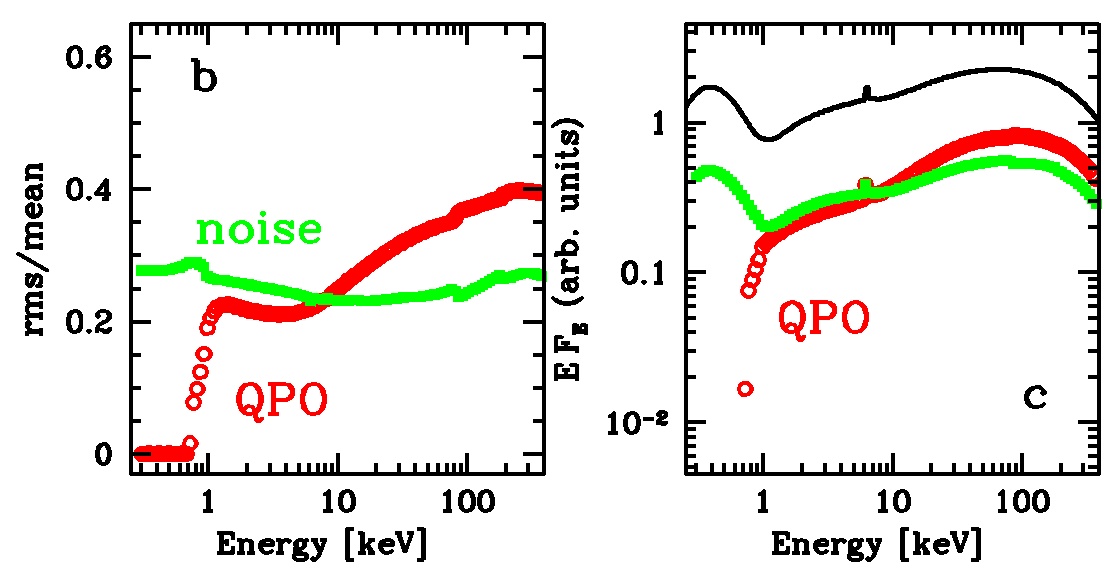
Now, assume that the heating rate of a plasma cloud is modulated periodically, while the cooling rate stays constant. Computing a sequence of spectra we get harder spectra when the ratio heating/cooling is larger, and softer spectra when the ratio is smaller. In other words, we obtain a specific pattern of spectral variability. The spectral variability produces a r.m.s.(E) relation, describing the amplitude of the variability as a function of energy. In this case the r.m.s. increases with energy, and the reason for this should be obvious from the plot to the right.

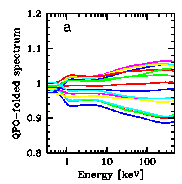
QPO period-folded spectra, divided by the time averaged spectrum. Amplitude of variability increases with energy.

Corresponding r.m.s.(E) relation is shown to the left (left panel). When multiplied by time-averaged spectrum, this gives something that can be thought of as the QPO energy spectrum. The important result here is that te QPO energy spectrum is harder than the time averaged spectrum.

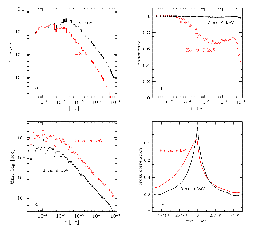
One can compute many other observable quantities, for example results of cross-correlation analysis between two different energy bands, to see if any features appear at the frequency of the QPO (here at 1 Hz). In this example, there is a local maximum in the equivalent width of the Fe Kalpha line, and the time lags between 3 and 9 keV lightcurves show rather complex behaviour around 1 Hz.

Imagine magnetic flares as the source of X-ray emission in accreting black holes. Actually, this is what we think is happening at high accretion rates. (“High” means here “too high for the cold disk to remain truncated far away from the black hole”, but it is hard to give one good number; let's say it's a few per cent of Eddington rate.) The magnetic flares rotate with the accretion disk, so the X-rays are modulated by relativistic effects. The main effect is obviously the Doppler effects, which enhance the emission from the part of the disk, which is going towards us, but reduce the emission from flares going away from us. Now, you've read this argument many times, but in most cases it was in connection with the broad profile of Fe Kalpha line, right? But the emission (both primary and reprocessed) is modulated in time, so what would we see, if we could observe the X-rays at sufficiently high time resolution?

This question was actually answered quite a few times in the past, in somewhat different contexts (Bardeen, Cuningham in the 1970s, Abramowicz and collaborators in 1980s).

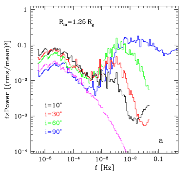
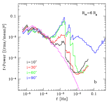
So, how does the time modulation look like? We computed the modulation of an intrinsically constant signal, emitted at 1.25 R_g (very close to the last stable orbit in extreme Kerr metric) and 6 R_g, as seen at 60 degrees inclination, for 10⁶ M_Sun (this sets the timescale). Below, on the left are the lightcurves, on the right – power spectra. The modulation is very strong, you cannot fail to notice it. Of course, it is periodic but far from sinusoidal, so there is a lot of harmonics in the PDS

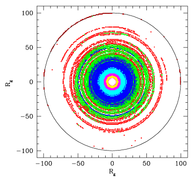
Of course, in a realistic situation we are not dealing with a single flare. We assume there is a lot of flares, longer and shorter (as required to explain the broad band power spectra in the flare avalanche model of Poutanen & Fabian 1999). Their radial distribution is such that the energy emitted follows the formula for an accretion disk around a Kerr black hole with a=0.998 – meaning simply that they are concentrated toward the center. All flares follow Keplerian orbits. After some time (about 10⁶ sec here) you see something like in the picture to the right: red means weak emission, green blue, cyan, magenta, yellow – progressively more (in log scale). The flares usually last longer than the orbital period (this is a requirement for the flare avalanche model; is it possible physically??), so each flare is modulated many times by the relativistic effects.

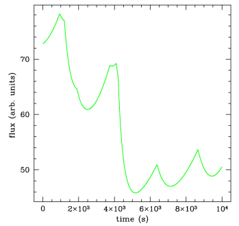
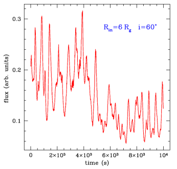
Compare the lightcurves: below, directly from the flare model, no relativistic effects, and right, with the relativistic effects included. The modulation adds a lot of power at high Fourier frequency.

And here come our main results: power spectra of such modulated signals.

The signal is rather obvious, isn't it? The magenta curve shows PDS of the intrinsic signal, without relativistic modulation. Of course, the modulation is stronger at higher inclinations. For Rin=1.25 Rg, it has so many harmonics that it all blends into a big bump, without any clear sharp peak. For Rin= 6 Rg you see peaks corresponding to the main frequency and one or two harmonics, at the innermost radius.

Would this be seen in real observations? Yes, it would. We simulated the data corresponding to recent XMM-Newton observations of MCG-60-30-15 (Vaughan et al. 2003) – count rate, duration, black hole mass 10⁶ MSun, inclination 30 degrees. And the modulation would be more than obvious in such data, if it was there. But it is not! Read more in our paper, how we did the simulations, and what exactly are the results.

This is basically a continuation of these two previous projects: fourier, fevar. This time I concentrate on the variability of the iron Kalpha line in the cold disk plus hot flow (“disrupted disk”) geometry. One one hand, this is motivated by those papers reporting that the Kalpha line in AGN is generally less variable that the continuum which drives it's emission, and it does not seem to correlate well with its driving continuum. On the other hand, it seems that we see an equivalent effect in Cyg X-1 and other black hole binaries: in the Fourier frequency resolved spectra the amplitude of reflection the EW of the Kalpha line get smaller with increasing Fourier frequency. Which means that the reprocessed component responds to the continuum variability on long time scales, but it does not do so on short time scales.

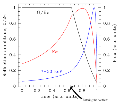
The decoupling of line and continuum variability in the propagation model in the disrupted disk geometry, are easy to understand. As an X-ray emitting structure (“active region”) propagates inwards, towards the central black hole, the X-ray flux increases. Initially, when the structure is above the “solid” part of the disk (red above), the relative amplitude of reflection is 1 (solid angle Omega=2pi). But when the structure enters the region below truncation radius, the emitted continuum flux still increases, but the reflection amplitude begins to decrease – simply because the disk “below” the structure is disrupted and so less effective in reprocessing. Since the flux of the Kalpha line is of course related to the amplitude, the flare of line flux peaks earlier than the fluxes of the continuum, and its amplitude is smaller. This is shown in the picture to the left, but note that the fluxes (line and continuum) were rescaled to 1 at peak. So this plot does not show correctly the relative amplitudes of the flare in the fluxes.

Now, it is a relatively simple matter to compute a sequence of spectra (in the same way as in previous project), and extract the flux of the Kalpha line and that of e.g. 7-30 keV continuum. Then, one can use the standard methods of cross-correlation analysis to see how the two fluxes correlate (or not), and compare those to correlations between two continuum bands. Some of the results are shown to the right.

Generally, you see reduced high-f variability (look at power spectra), lack of coherence, and longer time lags between the line and hard flux than timelags between two continuum bands. Interesting, isn't it? (read more)

Two main classes of geometries of accretion flows onto black holes are currently considered: a standard accretion disk truncated at certain radius and replaced by a hot, optically thin, geometrically thick flow (possibly an ADAF), or the standard disk extending to the last stable orbit, with either a dynamic corona or a hot skin. Each model has to be able to explain a range of X-ray spectral parameters (spectral slopes and amplitude of reflection), as well as correlations between them (e.g. the R-Gamma correlation; Zdziarski, Lubinski & Smith 1999).

The question is: is it possible to distinguish between the models (or at least learn something new about them) using timing, or correlated spectral-timing information?

I have decided to use the Fourier frequency resolved spectra for this purpose. The f-resolved spectra are energy spectra computed in a limited range of Fourier frequency (Revnivtsev, Gilfanov & Churazov 1999). That is, these are energy spectra of components varying on different time scales. The observed spectra show interesting dependence on f: the higher the frequency the harder the spectrum and the smaller the amplitude of reflection. 

In the geometry of an disrupted standard disk with inner hot flow one can imagine that the X-ray emission is produced by some sort of structures travelling from outside towards the center. These could be compact active regions related to, for example, magnetic reconnection and related particle acceleration during the flow (see the paper by Bisnovatyi-Kogan & Lovelace 2000). Alternatively, the active regions could be micro-shocks forming in the hot plasma as it accretes onto the center. Or, they could be global perturbations of the flow. Whatever they are, assume that the X-rays are produced at a rate roughly proportional to gravitational energy dissipation. A flare of radiation is generated, with rather slow rise and very sharp decay. As the flare progresses, the spectrum can be expected to evolve from softer to harder, simply because the supply of soft photons for Comptonization from the outer cold disk diminishes. Simultaneously, the instanteneous amplitude of the reprocessed component decreases, because the distant disk subtends smaller and smaller solid angle. This spectral evolution is precisely what is needed to produce the hard X-ray time lags (Kotov, Churazov & Gilfanov 2001).

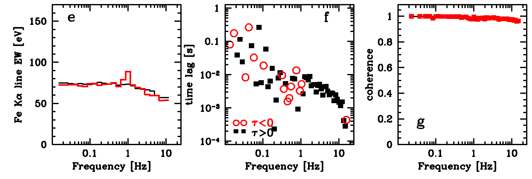
Given the geometry a number of observable quantities related to time variability can be computed. So the plot above shows (a) the f-resolved spectra (divided by a power law and normalized to 1 at 2 keV), (b) the equivalent width of the Fe Kalpha line as a function of Fourier frequency, and (c) time lags as a function of energy, for a number of Fourier frequency values. All of them agree with what is observed.

I have combined the variability model of Poutanen & Fabian (1999) with computations of the hot skin (see below) to compute the f-resolved spectra. The idea is that there is a unique correspondence between the flare's time scale and its position on the disk: fast (short lived) flares are located close to the center, while slower flares are located farther away. Since all parameters of the model of PF99 are uniquely specified if both energy spectra and timing properties (PSD, time lags) are to be quantitatively explained, so one can also uniquely compute the thickness of the hot skin, as a function of time, radius etc. The presence of the hot skin and a radial dependence of its thickness introduce a radial dependence of energy spectra.

The computations give an unexpected result: the (time averaged) thickness of the hot skin increases with radius. This is because the illuminating flux at the peak of a flare is the same for all flares, so it is constant with radius. Since the gravity decreases with radius, the thickness of the hot skin increases. (The same value of the peak flux for all flares is an important feature of the model and its modifications lead to wrong power spectra.) As a consequence, the fast flares (corresponding to high Fourier frequency) produce intrinsically softer energy spectra with larger amplitude of reflection. The slower flares (corresponding to low f) produce harder energy spectra with smaller amplitude of reflection. Correspondingly, the EW of the Fe K line increases with frequency. These results are opposite to what is observed in black hole binaries.

We computed the structure of the hot skin and underlying disk (the hot skin thickness does depend on the disk structure), as a function of irradiating flux. The conclusion is that is the flux increases by a certain factor, the thickness obviously does increases somewhat. This leads to a decrease of the line efficiency, which is however not sufficient to compensate the increase of the irradiation flux. The flux of line photons then does increase as a response to increased irradiation. If the irradiation flux is correlated with observed (no anisotropy), we cannot observe constant line flux when the continuum varies. There were later claims that the Fe line does vary on short time scales in MCG-6-30-15, but the variability is not easily related to the continuum variability. Perhaps the hot skin has some effect on the response of the line (well it surely should have), but it's not trivial - for example Sergei Nayakshin noticed that the adjustment of hydrostatic equilibrium when the medium is suddenly illuminated by a strong X-ray flux is relatively slow (on dynamical time scale). During the time the flux can change again, so the medium may be in a state not determined by the instantaneous X-ray flux. 

In upper panel the dashed contours represent X-ray flux, F - each contour means twofold increase of the flux. The solid (labelled) contours represent the relative amplitude of reflection, R. You can see that to get a decrease of R by e.g. a factor of 2, the flux must increase by much more than the factor of 2. This means that the flux of line photons, N \propto R * F, will not be constant when F changes 

We analyzed a number of data sets from archives, from old Ginga and newer RXTE satellites, for objects like GS 2000+25, GS 1124-68, GRO J1655-40, XTE J1550-564. This was of course not the first time that those data were analyzed, but we paid a bit more attention to the process of modeling, than was usually done before. First, in many papers the spectral features near 5-9 keV are modeled using so called 'smeared edge' model. That was useful 8-10 years ago when it was introduced, but even then K. Ebisawa remarked that the only reason to use it is that a proper, computationally efficient model of X-ray reprocessing did not exist. There is no such excuse now, when good models of reprocessing are available. In particular, it is important to use models which consistently compute the Compton-reflected continuum and the Fe Kalpha line.

Second, a simple power law is not the ideal model for the hard tail, if this is due to Comptonization of the soft photons from the thermal component: one has to use a model that includes the low energy cutoff (at the seed photons temperature about 1 keV) in the Comptonized spectrum. 

Residuals from a sequence of fits to Ginga data of GS 2000+25, showing that the best fit model (lowest panel) has a Comptonized soft component, second hard Comptonized component and its reprocessed component.

There are two main conclusions from modeling a number of spectra: 

1. the soft component seems to be more complex than previously thought. Phenomenologically, we can describe it either as a sum of a disk blackbody and an additional blackbody, or as a Comptonized blackbody (the data are not good enough to distinguish the two possibilities). So how do we interpret the two possibilities? 

The first could be that the disk blackbody is the usual thermal emission from the accretion disk, while the additional blackbody comes from hotter spots on the disk. The hot spots would be areas close to magnetic flares, illuminated by the hard X-rays (the hard tail) produced in the flares. If the flares are relatively compact (as they seem to be, Nayakshin & Kallman 2001), the illuminated area is relatively small and its temperature relatively high. 

The second possibility - Comptonized blackbody - would mean that the vertical structure of the disk is not trivial. For example the disk could have a hot skin (but rather thicker than what we considered in previous project! - Thomson thickness about 10), and so the soft photons coming from the disk interior would be additionally Comptonized 

Another related possibility is that the Comptonizing plasma has hybrid energy distribution of electrons (see the paper by P. Coppi). The low energy electrons have a Maxwellian distribution, so they do the low temperature thermal Comptonization, while the high energy electron have a power law (non-thermal) distribution, producing a power law photon spectra 

2. the proper reprocessed component very well describes the spectral features near 5-9 keV - no need for 'smeared edge' and gaussian line. The reprocessed component is highly ionized (that's what we would expect considering that the disk temperature is a good fraction of 1 keV - or even more). It also seems to be additionally smeared - that means the spectral features are even broader that what we would expect from superposition of a number of degrees of ionization. That suggests Doppler effect from the accretion disk, although it should be remembered that Comptonization of the spectral features, as the photons diffuse to the surface, is not properly modeled by most models of reprocessing. This may affect the results of spectral fitting. On the other hand, it's difficult to imagine that the reprocessor is so hot and located so far away from the center that the Doppler effect is unimportant

1. Zycki, Done & Smith, 1997, ApJ, 488, L113

2. Zycki, Done & Smith, 1998, ApJ, 496, L25

3. Zycki, Done & Smith, 1999, MNRAS, 305, 231

4. Done & Zycki, 1999, MNRAS, 305, 457

5. Done, Madejski & Zycki, 2000, ApJ, 536, 213

6. Di Salvo, Done, Zycki, Burderi, Robba, 2001, ApJ, 547, 1024

In these papers we analyzed a number of X-ray data sets from various objects (1., 3.- SXT GS 2023+338; 2.- SXT GS 1124-68; 4., 6.- Cyg X-1, 5. - Seyfert 1 IC 4329a) to try to characterize the X-ray reprocessed component. The reprocessed component consists of the Compton reflected continuum and spectral features superimposed on it. Of these spectral features the Fe Kalpha line and Fe K-shell absorption edge (roughly at 6-9 keV) are most prominent. Assuming the simple reprocessing model (uniform constant density medium) the properties of the line and the continuum are uniquely related. That is, when you've specified all the parameters needed to compute the reflected continuum, the Kalpha line is uniquely determined (so its energy, or energies of its components, and intensity is determined). Well, that is obvious if we think about it from the point of view of atomic physics. It is perhaps less obvious how to construct a good, computationally efficient model of such a reprocessed component. That is probably why the most popular reflection models implemented in XSPEC (pexrav and pexriv constructed by Magdziarz & Zdziarski; 1995) compute only the reflected continuum without the line. But simply adding to the continuum a gaussian line to account for the Kalpha line is not a good solution, since there is no way to ensure the consistency of the properties of the continuum and the line. It certainly did not work for us especially when the reprocessing was ionized and e.g. the energy of the line could not be fixed in the fitting procedure. So we implemented the model which computed the line consistently with the reflected continuum. The line was computed as in Zycki & Czerny (1994), with photoionization computations as in Done et al. (1992; the same code which is used in pexriv). We also added the possibility that the spectral features are broadened by Doppler effects and gravitational redshift, if they come from a rotating accretion disk (using the prescription from Fabian et al. 1989). Such a model has fewer free parameters than the "smeared edge" plus broad gaussian line model, and of course is superior to the latter since the parameters have physical meaning. And the reprocessed component can be computed for any (reasonable) primary continuum spectrum. Well, that much for the propaganda. The model is available for downloading here.

The results of modeling many datasets of various source (but all of them were in the low/hard state) was that:

• The reprocessed component is there, or, when the characteristic broad residuals are seen near 5-9 keV when you've fitted a power law to your data, the residuals can always be fitted by the reprocessed component.

• In low/hard state the reprocessed component is rather weakly ionized and its amplitude is less than 1 (where 1 means an isotropic source above a flat infinitely extended disk).

• The spectral features are additionally broadened ("smeared"). The smearing can be interpreted as the kinematic/relativistic effects from an accretion disk, but the inner radius of the disk is larger that the last stable orbit at 6 Rg (=6GM/c^2). This means that the reflecting disk does not go all the way to the last stable orbit, contrary to what we might expect.

These results are consistent with the idea that the accretion disk is truncated at somewhere between 20Rg and 100Rg, and, let's say, replaced by a hot X-ray producing flow (possibly an ADAF), but this is not a unique interpretation (see for example Di Salvo et al. 2001).

In GS 1124-68 (Nova Muscae 1991, paper 2.) we analyzed a number of datasets, which covered a part of the decline phase of the source outburst, namely a soft state, and the transition to the hard state. Very nice result that we obtained for the transition is that there is an evolution of not only the primary continuum, but also of the reprocessed component. Its amplitude decreases with time, and its ionization drops suddenly when the soft-to-hard transition takes place. The results for relativistic smearing were not unique. They were consistent with both an increasing value of the inner radius of the reflecting disk, but a constant Din could also describe the data. Overall then, these results were consistent with a retreating inner disk as the accretion rate was decreasing, in qualitative agreement with the ADAF-based models, but quantitatively the radii we derived were much smaller than those proposed in the ADAF papers.

The atmosphere of an illuminated accretion disk is unlikely to have a constant density. X-ray illuminated plasma under the condition of hydrostatic equilibrium is subject to the thermal instability. This makes the vertical structure of such disks quite complex, and computations of the reprocessed spectra from them very difficult. Computations of the vertical structure and resulting spectra were done by Agata Rozanska with collaborators and a good working model of the reprocessed component, ready for implementing into XSPEC, was constructed by S. Nayakshin. But the precise geometry of the reprocessor is still uncertain and it's not obvious a priori, which approximation (constant density of hydrostatic equilibrium) may be more appropriate. Whichever you choose, do it consistently.